Building A Transformer To Predict Stocks

2024-07-15

See part 1

Before we look at the model I still need to figure out why things are dying the moment we try to train - even on a simpler model. More process kills. This is undoubtedly due to memory again. The issue is that I don't really know if my data processing steps were successful. I have some options now. I can try and reduce memory further or I can move to a cloud solution. I suspect I'll need to resort to the latter eventually, but for now, let's see if we can reduce memory a bit more.

Memory loss

I don't want to reduce the number of features, compared to how I started my current features are practically anemic. So, just for testing, I'll reduce the number of stocks we're using. I downsized the dataset to around 1000 stocks, less than 1/5th of the total size of the dataset. This reduced our memory (for at least the training data) to around 30GB, and should limit how much it balloons during training. Success! We're training!

But there's a problem. As the first epoch starts processing I'm noticing the validation loss is increasing quickly, 30, 40, 70, 80, and then it turns to nan. Along with all of our other metrics. After a ton of debugging and tooling around I discovered the issue had to do with my not so brilliant idea to use float16. I was getting buffer overflows. So I had to go back to using float32. But memory was up to 60GB now. At this point, I'm not willing to reduce the number of stocks (it's a large model, so the dataset needs to be at least reasonably large). So, I'm going to have to move to a cloud solution.

In the clouds

I decided to use Paperspace. I've used it before to some success, and I honestly have limited patience for setting up something from scratch on AWS or GCP. I spun up a machine with 90GB of memory and an A100. This should do it. So we train again. This time no buffer overflows, but the process is still dying. It's memory again. The training process is going beyond the 90% memory utilization max and crashing. We're going to need a bigger boat. But those big boats are hard to come by. Once available, we're going to snag a 2xA100s (or an H100!) and see what we can do.

But until that time, let's talk about the (highly simplified due to memory constraints) model.

The model

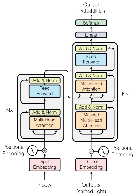
The model itself is a variation on the model described in Attention is all you need. You can generally get the idea of the model from following this excellent tutorial.

Looking at the model from the architecture diagram, I'll discuss some of the differences. The left side of the model is the encoder, which is responsible for taking the input data and learning relationships about itself. It builds a representation of the input data that learns the relationships between its own features - this is the whole premise behind self-attention. The right side of the model is the decoder. The decoder learns predictive relationships - so it only learns the relationships between each element and the elements that came before, and then combines this with the encoder output to generate a model that can make predictions that generate sequences of outputs, not just a single prediction. So, an encoder model would produce a single day of predictions, whereas an encoder-decoder model would produce many days of predictions.

For our purposes, because we are just trying to predict a single day, we can simplify this and just use an encoder, so our output will be a model that learns the relationships between the features of the input data alone. The decoder trains on the output data and crosses it with the input data, giving it some sense of longer term prediction. Using just an encoder is a simplification, but it will serve for our purposes. Maybe I'll build a decoder later.¹

The model (again)

def create_transformer_model(sequence_length, num_features, num_stocks, head_size, num_heads, ff_dim, num_transformer_blocks, ff_units, dropout=0.1):
    inputs = Input(shape=(sequence_length, num_features, num_stocks), dtype=tf.float32)

    x = ReshapeLayer([-1, sequence_length, num_features * num_stocks])(inputs)
    x = PositionalEncoding(sequence_length, num_features * num_stocks)(x)

    for _ in range(num_transformer_blocks):
        x = Encoder(head_size, num_heads, ff_dim, dropout)(x)

    x = GlobalAveragePooling1D().call(x)

    for dim in ff_units:
        x = FeedForward(dim, dropout)(x)

    outputs = Dense(num_stocks * 2, activation="linear",
                    kernel_regularizer=l2(0.01), dtype=tf.float16)(x)
    outputs = ReshapeLayer([-1, 2, num_stocks])(outputs)

    model = Model(inputs, outputs)
    model.compile(optimizer=tf.keras.optimizers.Adam(
        learning_rate=1e-4, clipnorm=1.0), loss='mse', metrics=[tf.metrics.RootMeanSquaredError()])

    return model

At a high level we're: adding a positional encoding, passing the result to a number of encoder blocks, pooling the data, and passing it through a feed forward layer.

Let's look at each of these components in turn. ²

Positional encoding

Unlike RNNs, transformers don't inherently have a sense of position. So, we need to give the transformer an understanding of how the data is ordered. We do this by adding position data to the input.

class PositionalEncoding(tf.keras.layers.Layer):
    def __init__(self, sequence_length, depth):
        super(PositionalEncoding, self).__init__()
        self.pos_encoding = self.positional_encoding(sequence_length, depth)

    def positional_encoding(self, sequence_length, depth):
        angles = self.get_angles(np.arange(sequence_length)[
                                 :, np.newaxis], np.arange(d_model)[np.newaxis, :], d_model)
        angles[:, 0::2] = np.sin(angles[:, 0::2])
        angles[:, 1::2] = np.cos(angles[:, 1::2])

        pos_encoding = angles[np.newaxis, ...]
        return tf.cast(pos_encoding, dtype=tf.float32)

    def get_angles(self, pos, i, depth):
        angle_rates = 1 / np.power(10000, (2 * (i // 2)) / np.float32(d_model))
        return pos * angle_rates

    def call(self, x):
        return x + self.pos_encoding[:, :tf.shape(x)[1], :]

A lot of this math is over my head, but we're basically creating a positional encoding for our data by adding sine and cosine waves whose frequencies are mapped to the position of the elements in the sequence. This assigns an order to our data, which is important for a time-series like our stock data.

Encoder

Now let's look at the encoder, this is where the magic happens.

class Encoder(tf.keras.layers.Layer):
    def __init__(self, head_size, num_heads, ff_dim, dropout=0.1):
        super(Encoder, self).__init__()
        self.head_size = head_size
        self.num_heads = num_heads
        self.ff_dim = ff_dim
        self.dropout = dropout

    def call(self, x):
        x = LayerNormalization(epsilon=1e-6, dtype=tf.float32)(inputs)
        x = MultiHeadAttention(
            key_dim=head_size, num_heads=num_heads, dropout=dropout, dtype=tf.float32)(x, x)
        x = Dropout(dropout, dtype=tf.float32)(x)
        res = x + inputs

        x = LayerNormalization(epsilon=1e-4, dtype=tf.float32)(res)
        x = Dense(ff_dim, activation="relu", kernel_regularizer=l2(0.01), dtype=tf.float32)(x)
        x = Dropout(dropout, dtype=tf.float32)(x)
        x = Dense(inputs.shape[-1], dtype=tf.float32)(x)

        return x + res

The attention layer (the MultiHeadAttention layer) on the encoder is the "global self-attention" layer. This is basically taking the entire input sequence and finding the most important segments of data. If you're still wondering what multi-head attention does, said another way, it's basically a way for a sequence of data to consider every other part of the sequence and weighting them based on their importance. As I mentioned, the novel part of this layer is that it's learning the relationships between itself and...itself (notice the (x, x) inputs on the attention layer). Voila, self-attention. The rest of the encoder is just a feed forward layer and some dropout.

More feed forward

Now that we a bunch of outputs from the various encoder blocks, we want to combine them and pass them through a feed forward layer.

class FeedForward(tf.keras.layers.Layer):
    def __init__(self, ff_dim, dropout=0.1):
        super(FeedForwardLayer, self).__init__()
        self.ff_dim = ff_dim
        self.dropout = dropout

    def call(self, x):
        x = Dense(self.ff_dim, activation="relu", kernel_regularizer=l2(0.01), dtype=tf.float32)(x)
        x = BatchNormalization(dtype=tf.float32)(x)
        x = Dropout(self.dropout, dtype=tf.float32)(x)

        return x

And the output is a model we can use to predict stock prices.

All of this is governed by a few hyperparameters:

• head_size: The size of the heads in the transformer blocks
• num_heads: The number of heads in the transformer blocks
• ff_dim: The size of the feed forward layer in the transformer blocks
• num_transformer_blocks: The number of transformer blocks
• ff_units: The number of dense layer blocks and their sizes

We can fiddle with these to change the complexity of the model.

Here's some very small hyperparameters that we can use to test the training process and make sure we're getting at least some kind of reasonable result:

head_size = 16
num_heads = 2
ff_dim = 16
num_transformer_blocks = 2
ff_units = [32, 16]
dropout = 0.1

This is a very small model, but it should at least train. "Should" is the operative word here. But operative doesn't always mean "will". And in this case, it does not. Even with reasonable parameters this model is too big. There's no doubt I'm going to need more memory. But I'll have to wait until I can get more GPUs provisioned.

Thoughts on LLMs

It's kind of incredible how big these models are. The "Large Language Model" name is really no joke. Even a relatively small model like the one we're trying to train here is pretty large.³ And this is with a fraction of the complete dataset. Even with this small model and the reduced dataset we're not only running into memory issues, but it takes about an hour to train and test using KFold cross validation (with k=5). Using the full sized model with a complete dataset would take dozens hours to train once. And we'd need to tune the hyperparameters. Which is potentially hundreds of runs of the training process that get progressively longer with increased model complexity. I tested out timing using a more complex model, and even with only 5 features it still took many hours to complete one full run.

And the cost!⁴ Let's say I'm exaggerating and we're able to tune the full model in 20 runs. Let's also say that the full sized model only takes 10 hours to train (it's much longer than this in reality). That's 200 hours of training. At a cost of around $6/hour per H100 GPU with 268GB RAM, and a need for probably 5 of those (remember the model was 700GB+ and we need a lot of headroom for training), that's ~$30/hour to train the model, or $6,000. This is a mega lowball estimate. But it's still not cheap for a hobby project. For more serious projects I suspect training costs are in the tens of thousands of dollars. That's not including the cost to host the model and perform inference.

There's a strange dichotomy then. It's actually not that hard to build a model like this - with a few open source libraries it's pretty accessible. But actually training it and utilizing it is inaccessible to most. With this framing, it's easy to see why compute resources are the picks and shovels of this AI gold rush.

But wait, there's more

Okay, so I gave in and decided to remove some more features. I decided to try things out only using open, high, low, close, volume, rsi, fft, and wavelet approximation features. I also reduced the number of training epochs to 10. And still no dice. I reduced the features even further to only use open, high, low, close, and fft and it trained! Here are the results:

These results aren't great. Particularly our MAPE, which is a measure of the average percent error.⁵ A value of 231 means we are, on average, 231% off. Yikes. But that's okay, we have something that actually runs that we can improve upon. Which is the next step of our journey, feature engineering and fine tuning (likely with some model re-architecture)!

But I'm going to revel in my success here. I have technically trained an transformer model that predicts stock prices. It doesn't get them right, but it predicts them nonetheless! Please don't use this. You will definitely lose money.