
Profitable trading with mean reversion
2024-07-19
We've been talking a bit about using models for predicting stock prices, but we haven't really talked much about trading strategy. Instead, we've implemented a simple strategy of:
- Buy with our entire bankroll when the next day's closing price is predicted to be higher
- Sell everything when the next day's closing price is predicted to be lower
This is a highly simplistic strategy and doesn't really take into consideration the benefits of actually making an accurate prediction.
This time, we're going to put aside the notion of prediction and consider a common algorithmic trading strategy called mean reversion. The concept is that if a stock price deviates too far from its mean, it will eventually revert back to the mean. Fundamentally, this is untrue. Stock prices do not tend to be mean reverting. However, we can pull a few tricks by combining, or cointegrating assets within a portfolio to create a mean reverting spread. But lets start with the basic concept of mean reversion.
Linear mean reversion
The basic concept of mean reversion is that if a price is deviates from the mean, it will eventually revert. But there's an underlying question, how do we know when to buy (or sell)?
There are a few strategies here, but we'll use a simple one. Determine the mean (we'll use a simple moving average [SMA] here) and standard deviation of the price so far, and then scale our ownership of the asset based on the standard deviation from the mean. We'll add a proportionality constant $k$ (10,000 works well for our use case here) so our ownership of a stock will be proportional to the negative deviation from the mean:
$ownership = -k * \dfrac{price - SMA}{\sigma}$
Where $k$ is our constant, $SMA$ is our mean, and $\sigma$ is our standard deviation. If the price is below the average, we'll own an amount of the stock, if it's above the average, we'll short/sell an amount of the stock.
Let's implement this in code.
import pandas as pd
window = 5

data['SMA'] = data['Close'].rolling(window=window).mean()
data['Std'] = data['Close'].rolling(window=window).std()

data['Normalized_Deviation'] = (data['Close'] - data['SMA']) / data['Std']
data['Ownership'] = -data['Normalized_Deviation'] * 10000

data['Action'] = data['Ownership'].diff().fillna(0)
Now, let's test this out with some real data. We'll look at AMD (AMD) and Micron Technology (MU).
After executing our trading strategy, this is what our portfolio values look like for AMD and MU:
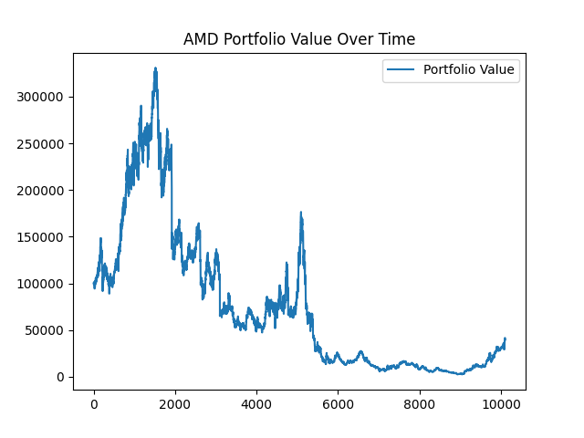
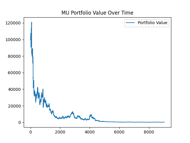
With MU, our portfolio goes to $321! From $100,000! That's horrible. For AMD it's a little better, we go from $100,000 to $39,934. With both of these stocks we see a significant loss while executing our mean reversion strategy.
Why did this fail? Well, the answer should be fairly obvious. Stocks don't actually tend to revert to the mean. Or said another way, they are not stationary. Let's take a look at both stocks during this time period:
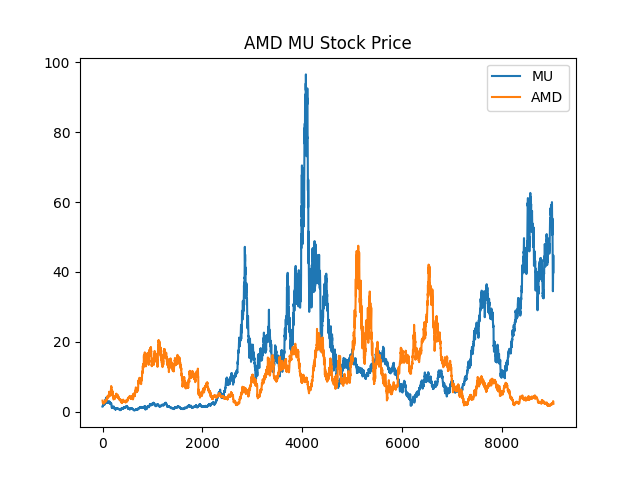
These prices generally don't display much of a trend.1 But we don't have to eyeball this. We can measure its stationarity by running a Augmented Dickey-Fuller test. The test is a statistical test, so it's testing the null hypothesis of non-stationarity. If the probability is less than 0.05, we can reject the null hypothesis and say that the data is stationary.
from statsmodels.tsa.stattools import adfuller

result = adfuller(data['Close'])
Let's run the tests on AMD and MU.
| ADF test statistic | p-value | 1% | 5% | 10% |
|---|---|---|---|---|
| -2.8258 | 0.0547 | -3.4310 | -2.8612 | -2.5669 |
AMD ADF test
| ADF test statistic | p-value | 1% | 5% | 10% |
|---|---|---|---|---|
| -2.5886 | 0.0954 | -3.4311 | -2.8619 | -2.5669 |
MU ADF Test
For AMD, we have a p-value of 0.0547, which is just barely is greater than 0.05, so we fail to reject the null hypothesis. For MU, the p-value of 0.0954 is also greater than 0.05, which means we also fail to reject the null hypothesis. Both stocks being non-stationary demonstrates why our mean reversion strategy is doomed to fail.
So is mean reversion useless? Not so fast. We were only considering each stock on its own. What if we considered both stocks in a hedged strategy that, when combined, were stationary? This is the magic of cointegration.
Cointegration
Cointegration is the idea that two or more non-stationary time series can be combined to create a stationary one. Typically, this is done by going long on one stock and short on another to create a cointegrated portfolio that will have a stationary spread. If the spread eventually reverts to the mean, we can use the mean reversion strategy to profit.
We're going to look at these stocks (AMD and MU), mainly because they're in the same sector - it's easier to find cointegrated equities within the same industry. Let's first look at a scatter plot of the two stocks to see if they are good candidates for cointegration.
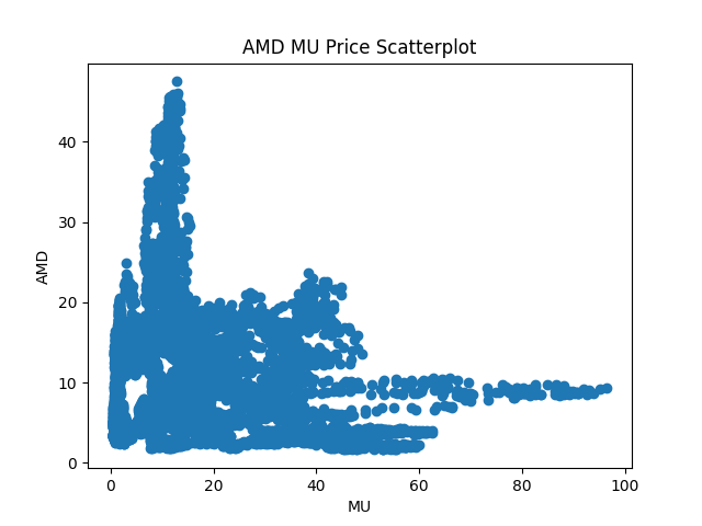
This looks okay, but not great. There is clearly some sort of relationship here, but it's unclear whether it's linear. Let's move forward and we'll test for stationarity in a bit. For now, we'll use an Ordinary Least Squares (OLS) regression to determine the hedge ratio between the two stocks.
import pandas as pd
from statsmodels.api import OLS, add_constant
    symbol1 = 'AMD'
    symbol2 = 'MU'

    symbol1_data = get_data(symbol1)
    symbol2_data = get_data(symbol2)

    prices1 = symbol1_data['Close'].rename(symbol1)
    prices2 = symbol2_data['Close'].rename(symbol2)

    combined_data = pd.merge(prices1, prices2, left_index=True, right_index=True, how='inner')
    stock1 = combined_data[symbol1]
    stock2 = combined_data[symbol2]

    returns1 = stock1.dropna()
    returns2 = stock2.dropna()

    returns2 = add_constant(returns2)

    model = OLS(returns1, returns2).fit()

    hedge_ratio = model.params[0]
And we get a value of 1.27. This means that to hedge one unit of AMD, we need to short ~1.3 units of MU.
Now we'll run a cointegrated ADF (CADF) test2 to see if the spread of the two stocks are stationary, and therefore cointegrated.
from statsmodels.tsa.stattools import adfuller

combined_data['Spread'] = stock1 - hedge_ratio * stock2
cadf_result = adfuller(combined_data['Spread'].dropna())
The results are as follows:
| ADF test statistic | p-value | 1% | 5% | 10% |
|---|---|---|---|---|
| -3.5494 | 0.0068 | -3.4311 | -2.8619 | -2.5669 |
AMD and MU spread
The p-value of 0.0068 is less than 0.05, so we can reject the null hypothesis that the data is not stationary. This means that the spread between AMD and MU is stationary and cointegrated. A graph of the spread demonstrates this as well.
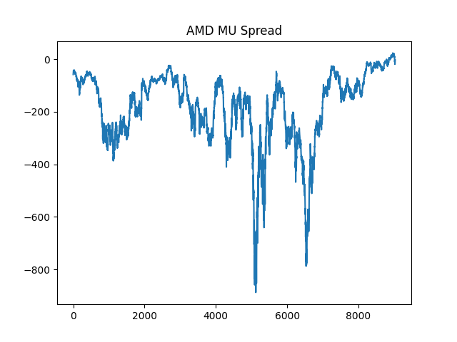
This means we can potentially use a mean reversion strategy to profit.
Let's put everything together and modify our mean reversion strategy to use the spread between AMD and MU.
def cointegrated_mean_reversion_strategy(symbols, symbol_data, window=5):
    symbol1, symbol2 = symbols
    symbol1_data, symbol2_data = symbol_data

    prices1 = symbol1_data['Close'].rename(symbol1)
    prices2 = symbol2_data['Close'].rename(symbol2)

    combined_data = pd.merge(prices1, prices2, left_index=True, right_index=True, how='inner')[:1000]
    stock1 = combined_data[symbol1]
    stock2 = combined_data[symbol2]

    returns1 = stock1.dropna()
    returns2 = stock2.dropna()

    returns2 = add_constant(returns2)
    model = OLS(returns1, returns2).fit()

    hedge_ratio = model.params[0]

    combined_data['Spread'] = stock1 - hedge_ratio * stock2

    combined_data['SMA'] = combined_data['Spread'].rolling(window=window).mean()
    combined_data['Std'] = combined_data['Spread'].rolling(window=window).std()

    combined_data['Normalized_Deviation'] = (combined_data['Spread'] - combined_data['SMA']) / combined_data['Std']
    combined_data[f"{symbol1}_Ownership"] = -combined_data['Normalized_Deviation'] * 10000
    combined_data[f"{symbol2}_Ownership"] = combined_data['Normalized_Deviation'] * 10000
    combined_data[f"{symbol1}_Action"] = combined_data[f"{symbol1}_Ownership"].diff().fillna(0)
    combined_data[f"{symbol2}_Action"] = combined_data[f"{symbol2}_Ownership"].diff().fillna(0)

    return combined_data
We're basically doing the same thing we did before, this time modifying the ownership of each stock based on the spread between the two stocks. We'll then backtest this strategy just as before. I shortened the time period to 1000 days to the chart is more visible. After executing our trading strategy, this is what our portfolio value looks like:
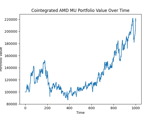
Not bad! We went from $100,000 to $217,206 in 1000 days. That's an annualized rate of return of 32.74%. That's great.3
Conclusions
This is a fairly simple strategy that can be improved upon. But there are some nice qualities to its simplicity. Cointegration is fairly logical, and you can reason about assets that are cointegrated. But there are some pitfalls as well. Just because two assets are cointegrated doesn't mean they will stay cointegrated. Things can quickly fall off without much notice. So, deploying a mean reversion strategy requires quite a bit of risk management. But if you manage risk effectively, mean reversion can be one good component of a quantitative trading strategy.4
This goes to show that you don't necessarily need machine learning to devise a profitable trading strategy. But. If we have it, we can potentially supercharge simple strategies such as this. Maybe I'll explore that in the future.
-
AMD actually looks like it somewhat exhibits a trend, but those big peaks are very likely to throw off the mean, especially given that we're using a simple moving average. This inherently disrupts mean reversion. Our eventual ADF test demonstrates that while AMD is close to stationarity, it just barely isn't. This small effect clearly disrupts the effectiveness of a mean reversion strategy, as demonstrated. ↩
-
The cointegrated ADF only works for a portfolio comprising a pair of stocks. You absolutely can create a portfolio of multiple stocks (there really is no limit) but you have to run a different statistical test, such as the Johansen test, to determine stationarity. ↩
-
I cheated here. I only show the first 1000 days of data, but if you extend this strategy further, eventually these two stocks are no longer cointegrated and the strategy will fail. This is a common pitfall of mean reversion strategies. They are not always stationary. ↩
-
The trading strategies discussed here are for illustrative purposes only and are not meant to be used in a live trading environment. They are not investment advice and should not be used as such. ↩