
Some baseline models for stock prediction
2024-08-07
As I develop my transformer model for stock prediction it's important to have some baselines for comparison. There are many ways to predict stocks out there and most of the accurate ones are likely shrouded in secrecy. But there are a number of simple models that can be used as baselines and benchmarks. We're going to spend some time looking at these models and running them through some backtesting to see just how powerful they are and what our transformer is up against.
We're going to be training our models, using them for prediction, and then using those predictions in a simple backtesting exercise. Our strategy will be very simple. We'll start with $10,000 in our portfolio, if the model predicts the stock will go up, we'll buy the stock with all of our cash. If it predicts the stock will go down, we'll sell all of our holdings if we have any. We'll keep track of our profits and losses and see how we do. Here's the strategy we'll be using:
def backtest(data, predictions, initial_cash=10000):
    cash = initial_cash
    holdings = 0
    cash_history = [cash]
    holdings_history = [holdings]

    signals = generate_signals(predictions)

    for i in range(len(signals)):
        if signals[i] == 'buy' and cash > 0:
            holdings += cash / data[i]
            cash = 0
        elif signals[i] == 'sell' and holdings > 0:
            cash += holdings * data[i - 1]
            holdings = 0

        cash_history.append(cash)
        holdings_history.append(holdings * data[i])

    total_value = np.array(cash_history) + np.array(holdings_history)
    return total_value


def generate_signals(predictions, threshold=0.01):
    signals = []
    for i in range(len(predictions) - 1):
        if predictions[i+1] > predictions[i] * (1 + threshold):
            signals.append('buy')
        elif predictions[i+1] < predictions[i] * (1 - threshold):
            signals.append('sell')
        else:
            signals.append('hold')
    return signals
We generate our buy/sell/hold signals by looking at the difference between the current day's prediction and the next day's prediction. If the next day's prediction is greater than the current day's prediction by a certain threshold, we buy. If it's less than the current day's prediction by a certain threshold, we sell. Otherwise, we hold. We'll use a threshold of 1%.
We're also going to be doing our prediction a little bit differently. While our transformer model is designed to predict many stocks at the same time, we're going to have our baselines only predict one stock at a time. This is because the models we're using are not designed to predict multiple stocks at once. We'll be using the closing price of the stock as our feature. We're going to be using a sequence length of 60 days. This means we'll be using the closing price of the stock for the last 60 days to predict the closing price of the stock for the next day. We'll be using the mean RMSE, MAE, and MAPE as our performance metrics.
LSTM
A simple LSTM (long short-term memory) model is one of the most common time series prediction models you'll find on the internet. These days they're easy to build, they're easy to train (they're not super data intensive), and they achieve relatively good performance.
A brief background on LSTMs. They're a type of recurrent neural network that is designed to remember long term dependencies. They do this by having a "memory cell" that can store information for long periods of time. This memory cell is controlled by a series of gates that determine when to read from the memory cell, when to write to the memory cell, and when to forget the memory cell. This allows the LSTM to remember patterns that occurred a long time ago and use them to make predictions. So, in short, they remember patterns and recall them to make predictions. But to be honest, this day and age we don't really have to understand much about what's going on under the hood (though it helps!).
Let's see how to build one.
 model = tf.keras.models.Sequential([
        tf.keras.layers.Input(shape=(sequence_length, num_features)),
        tf.keras.layers.LSTM(128, return_sequences=True),
        tf.keras.layers.LSTM(128),
        tf.keras.layers.Dropout(0.2),
        tf.keras.layers.Dense(num_features)
    ])
That's it. We define our input shape, add two LSTM layers, a dropout layer, and a dense layer. We're ready to train.
You'll notice this model is a bit different, in that it takes one stock rather than a full set of stocks. This model operates in a fundamentally different way than the transformer model we're building. Here, we're just learning the patterns of a single stock, while the transformer attempts to learn relationships between multiple stocks. But don't underestimate the humble LSTM. It's a powerful model that can learn a lot about a single stock. Even more simply, we're going to only use the closing price of the stock as our feature. Remember, we're trying to establish a set of simple baselines.
Let's see how it performs. We'll train it on a single stock and see how it does. We're going to train it on AAPL, with a sequence_length of 60 days. We'll use KFold cross-validation and see how it does on raw predictions and how it does using our simple trading strategy.
| Mean RMSE | Mean MAE | Mean MAPE |
|---|---|---|
| 0.006325 | 0.003369 | 17.112548% |
Our model performed admirably. It achieved a MAPE of 17.11%. Let's see how it does in our backtesting.
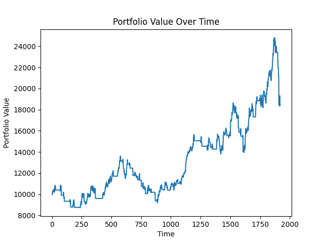
Not bad, but not great. Our LSTM model achieved a final portfolio value of around $18,000. Over 2000 days that's an annualized rate of return of 11.33%. Pretty good, but not for a stock that shot up thousands of percent over the same period. Let's see what the next model can do.
GRU
GRUs (gated recurrent unit) are another type of recurrent neural network that are similar to LSTMs. It's designed to remember long term dependencies, but it's a bit simpler than LSTM. It has fewer gates and is less computationally intensive to train.
    model = tf.keras.models.Sequential([
        tf.keras.layers.Input(shape=(sequence_length, num_features)),
        tf.keras.layers.GRU(128, return_sequences=True),
        tf.keras.layers.GRU(128),
        tf.keras.layers.Dropout(0.2),
        tf.keras.layers.Dense(num_features),
    ])
Looks pretty similar, doesn't it? Let's take a look at the results:
| Mean RMSE | Mean MAE | Mean MAPE |
|---|---|---|
| 0.005326 | 0.002654 | 13.177665% |
This model performed even better than the LSTM, achieving a MAPE of 13.18%. Let's see how it does in our backtesting.
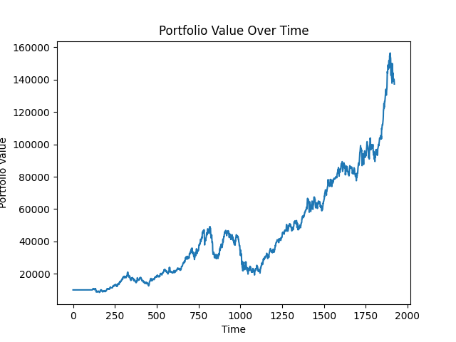
Outstanding performance. With just a small improvement in MAPE, our GRU model achieved a final portfolio value of around $140,000. That's an annualized rate of return of 33.5%. That's incredibly good. It's likely that directional accuracy was significantly better than the LSTM and the model took advantage of AAPL's skyrocketing value.
Random forest
Random forests are a bit different from LSTMs and GRUs. They are an ensemble learning method that operates by constructing a multitude of decision trees at training time and outputting the class that is the average prediction of the individual trees. They're a bit simpler than LSTMs and GRUs, but they can achieve good performance on time series data. However, they're not time-aware like LSTMs and GRUs. So we'll need to do some feature engineering to make them time-aware.
def create_features(data, sequence_length):
    df = pd.DataFrame(data)
    columns = [df.shift(i) for i in range(sequence_length)]
    df = pd.concat(columns, axis=1)
    df.dropna(inplace=True)

    return df
Here we're just shifting the data by sequence_length days and concatenating it into a single dataframe. This will allow the random forest to learn from the past sequence_length days. Now we just create the model:
model = RandomForestRegressor(n_estimators=100)
Very exciting, isn't it?
Let's see how we do.
| Mean RMSE | Mean MAE | Mean MAPE |
|---|---|---|
| 1.543903 | 0.716665 | 17.40063% |
The model performed okay. It achieved a MAPE of 17.4%. Let's see how it does in our backtesting.
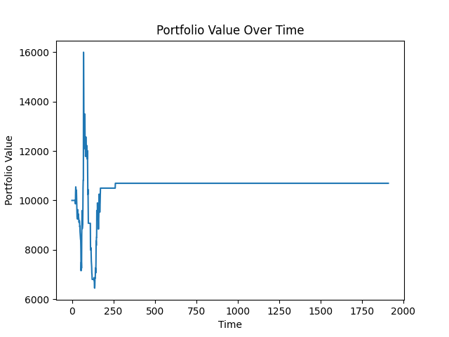
Not great. Our portfolio value ended up at little more than $10,000. As one might think, an annualized rate of return of 0% isn't exciting. One thing that may help is to add more features to the Random Forest, as it can be fairly powerful with the right features. So let's try again with some more features. We'll add volume, open, high, and low.
| Mean RMSE | Mean MAE | Mean MAPE |
|---|---|---|
| 2.029957 | 0.900653 | 24.90479% |
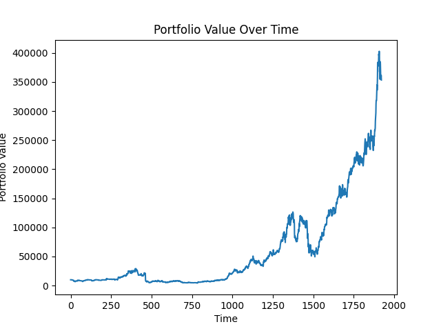
Wow, that's more like it. Our portfolio value ended up at around $360,000. Over 2000 days that's an annualized rate of return of 45%. These additional features clearly led to a different strategy, but it's important to note that it's not super exciting and that the performance metrics are actually worse than previous models. The strategy was simply buy and hold and let AAPL shoot to the moon. It's not a strategy that's likely to work on other stocks. This is something we'll need to test.
Shotgun testing
This isn't an official term, but we want to test how these models do on other stocks as well. AAPL has the distinguished honor of being one of the best performing stocks over the last 20 years. If you bought and held AAPL in 2000, you're probably a millionaire, so we're going to choose a few stocks randomly from our pool of 5800 and see how these models do.
Our random sample picked out IHC, ROKU, EC, DKL, and KXIN. Let's see how they do.
LSTM
| Ticker | Mean RMSE | Mean MAE | Mean MAPE | Portfolio Value |
|---|---|---|---|---|
| IHC | 5.243021 | 3.997438 | 47.97126% | $27,907.00 |
| ROKU | 35.67473 | 28.16644 | 33.99546% | $28,071.61 |
| EC | 10.21720 | 7.945024 | 26.47628% | $4,227.41 |
| DKL | 5.967252 | 4.974503 | 16.63728% | $9,704.91 |
| KXIN | 2.515743 | 2.039172 | 53.66002% | $9,062.92 |
GRU
| Ticker | Mean RMSE | Mean MAE | Mean MAPE | Portfolio Value |
|---|---|---|---|---|
| IHC | 1.914841 | 1.180831 | 14.62259% | $4,278.36 |
| ROKU | 27.01341 | 22.51532 | 33.83084% | $28,046.13 |
| EC | 5.466211 | 3.814912 | 16.12056% | $3,326.42 |
| DKL | 4.807646 | 3.414974 | 12.78373% | $6,820.67 |
| KXIN | 2.61506 | 1.065932 | 50.43762% | $9,482.42 |
Random Forest
| Ticker | Mean RMSE | Mean MAE | Mean MAPE | Portfolio Value |
|---|---|---|---|---|
| IHC | 1.703894 | 1.041218 | 16.69719% | $5,079.99 |
| ROKU | 28.608459 | 20.739215 | 32.75787% | $13,078.20 |
| EC | 6.45644 | 4.400034 | 14.86171% | $6,876.81 |
| DKL | 4.054983 | 3.031580 | 9.38363% | $11,034.30 |
| KXIN | 2.752207 | 1.285057 | 38.63279% | $10,000.00 |
Thoughts
Well, I have a good haul of baseline data from which to compare our transformer. It's worth noting that these models are more or less "raw". I did very little tuning and hyperparameter optimization. There was little thought in feature engineering. These are not optimal models for the task. But the point is that our transformer needs to perform better than these baseline models. If it doesn't, it's not worth pursuing too hard, especially given how much effort transformers take to train and tune. But our transformer has some distinct advantages over these baselines. For one, these models struggled to apply patterns they learned from one stock to another set of stocks - that's because they were only trained on one highly successful stocks. Other stocks were not so successful. Our transformer will be trained on a large set of stocks and will learn not only a different set of patterns, but the relationships between those patterns. My hope is that the transformer is then more flexible to volatility and our simple trading strategy can take effective advantage.
But it's worth noting how powerful these baseline model are, even in their not so optimal form. For each one, I was able to architect a model in a few minutes that achieved slightly more than mediocre results. It's likely these can be improved substantially.
I'm excited to see how our transformer does. Stay tuned for that.